from functools import partial

import matplotlib.pyplot as plt
import numpy as np
from scipy.spatial.distance import pdist
from scipy.stats import multivariate_normal

from frouros.callbacks import PermutationTestDistanceBased
from frouros.detectors.data_drift import MMD
from frouros.utils.kernels import rbf_kernel
Two bivariate normal distributions#
In order to show a simple example of the detection of samples coming from different distributions, two bivariate normal distributions are defined.
The first one is defined as follows:
x_mean = np.ones(2)
x_cov = 2 * np.eye(2)
print(f"x_mean = {x_mean}\nx_cov = {x_cov}")
x_mean = [1. 1.]
x_cov = [[2. 0.]
 [0. 2.]]
While the second is defined as follows:
y_mean = np.zeros(2)
y_cov = np.eye(2) + 1
print(f"y_mean = {y_mean}\ny_cov = {y_cov}")
y_mean = [0. 0.]
y_cov = [[2. 1.]
 [1. 2.]]
Some samples are generated for both distributions. \(N_{x}\) samples will be used as reference, while \(N_{y}\) samples will be used to test.
seed = 31
np.random.seed(seed)

num_samples = 200

X_ref = np.random.multivariate_normal(
    mean=x_mean,
    cov=x_cov,
    size=num_samples,
)
X_test = np.random.multivariate_normal(
    mean=y_mean,
    cov=y_cov,
    size=num_samples,
)
The Hypothesis Test can be defined as follows:
with a significance level of \(\alpha = 0.01\).
alpha = 0.01
In order the check if samples belong to the same distribution or not, Maximum Mean Discrepancy (MMD) [1] imported from Frouros is used with a Radial Basis Function kernel (RBF), set by default in MMD. In addition to calculating the corresponding MMD statistic, p-value is estimated using permutation test. According to [1], the recommended value for \(\sigma\) using an RBF kernel is the median distance between points in the aggregate sample. Therefore, \(\sigma = \dfrac{median(X)}{2}\), where \(X\) is the combined sample from \(N_{x}\) and \(N_{y}\).
sigma = (
    np.median(
        pdist(
            X=np.vstack((X_ref, X_test)),
            metric="euclidean",
        )
    )
    / 2
)
sigma
np.float64(1.2590251585463998)
Note: \(N_{y}\) samples cannot always be had before using the MMD fit, so \(\sigma\) would have to be selected in another way. In this case we assume that we have the \(N_{y}\) samples at the same time as the \(N_{x}\) samples.
detector = MMD(
    kernel=partial(
        rbf_kernel,
        sigma=sigma,
    ),
    callbacks=[
        PermutationTestDistanceBased(
            num_permutations=1000,
            random_state=seed,
            num_jobs=-1,
            method="exact",
            name="permutation_test",
            verbose=True,
        ),
    ],
)
detector.fit(X=X_ref)
mmd, callbacks_log = detector.compare(X=X_test)
p_value = callbacks_log["permutation_test"]["p_value"]
  0%|          | 0/1000 [00:00<?, ?it/s]
 62%|██████▎   | 625/1000 [00:00<00:00, 6203.75it/s]
100%|██████████| 1000/1000 [00:00<00:00, 5993.34it/s]
print(f"MMD statistic={round(mmd.distance, 4)}, p-value={round(p_value, 8)}")
if p_value <= alpha:
    print(
        "Drift detected. "
        "We can reject H0, so both samples come from different distributions."
    )
else:
    print(
        "No drift detected. "
        "We fail to reject H0, so both samples come from the same distribution."
    )
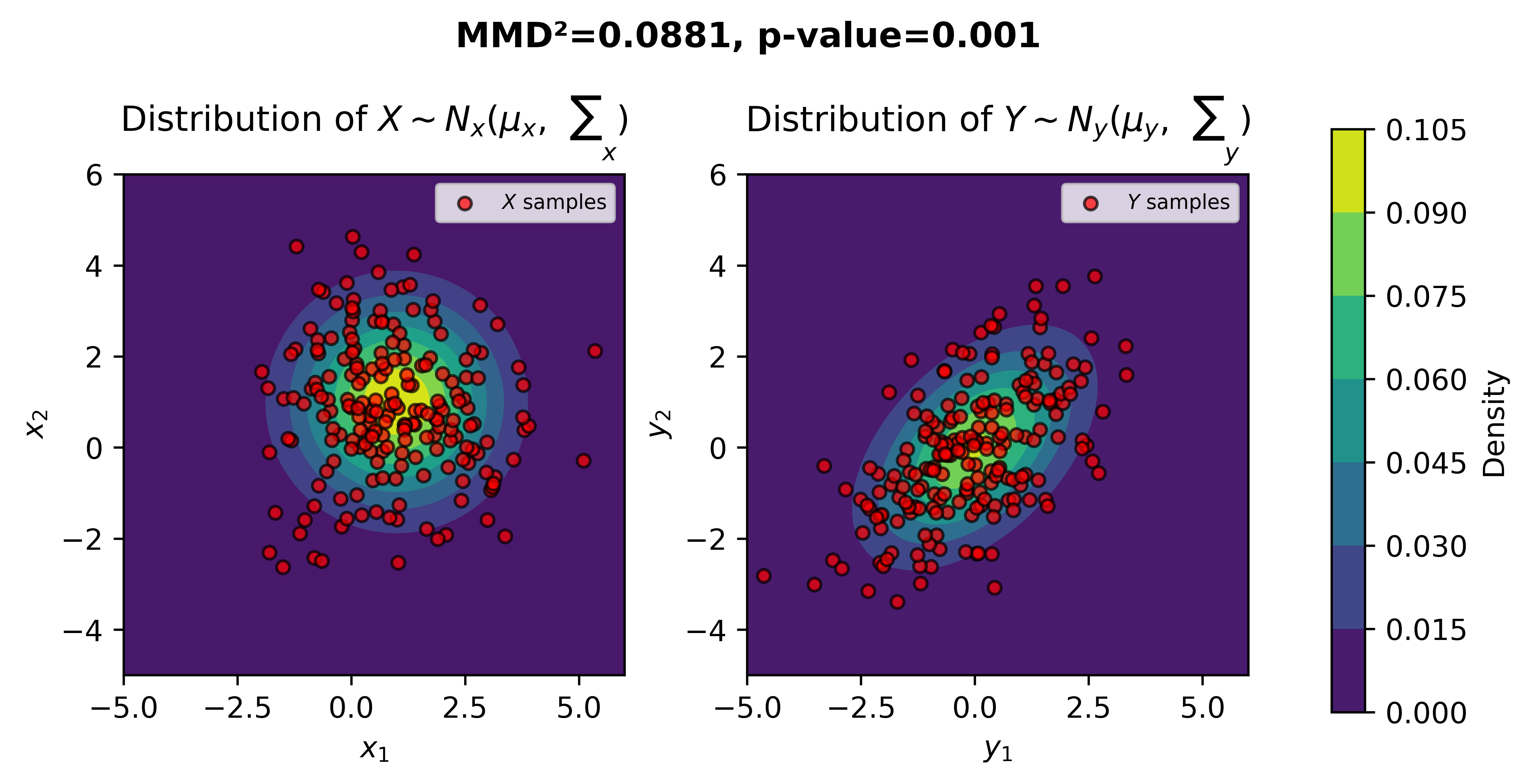
MMD statistic=0.0881, p-value=0.0009985
Drift detected. We can reject H0, so both samples come from different distributions.
Finally, we can visualize both samples with their respective distributions.
fig, (ax1, ax2) = plt.subplots(nrows=1, ncols=2, figsize=(8, 4), dpi=600)

x1_ref_min, x2_ref_min = X_ref.min(axis=0)
x1_test_min, x2_test_min = X_test.min(axis=0)

x1_ref_max, x2_ref_max = X_ref.max(axis=0)
x1_test_max, x2_test_max = X_test.max(axis=0)

x_min = np.floor(np.min([x1_ref_min, x1_test_min, x2_ref_min, x2_test_min]))
x_max = np.ceil(np.max([x1_ref_max, x1_test_max, x2_ref_max, x2_test_max]))
x_max = x_max if x_min != x_max else x_max + 1

x1_val = np.linspace(x_min, x_max, num=num_samples)
x2_val = np.linspace(x_min, x_max, num=num_samples)

x1, x2 = np.meshgrid(x1_val, x2_val)

px_grid = np.zeros((num_samples, num_samples))
qy_grid = np.zeros((num_samples, num_samples))

for i in range(num_samples):
    for j in range(num_samples):
        px_grid[i, j] = multivariate_normal.pdf([x1_val[i], x2_val[j]], x_mean, x_cov)
        qy_grid[i, j] = multivariate_normal.pdf([x1_val[i], x2_val[j]], y_mean, y_cov)

marker = "o"
facecolor = "r"
edgecolor = "k"
alpha = 0.7
marker_size = 20

CS1 = ax1.contourf(x1, x2, px_grid)
ax1.set_title("Distribution of $X \sim N_{x}(\mu_{x}, \sum_{\qquad x})$", pad=15)
ax1.set_ylabel("$x_2$")
ax1.set_xlabel("$x_1$")
ax1.set_aspect("equal")
ax1.scatter(
    X_ref[:, 0],
    X_ref[:, 1],
    label="$X$ samples",
    marker=marker,
    facecolor=facecolor,
    edgecolor=edgecolor,
    alpha=alpha,
    s=marker_size,
)
ax1.legend(fontsize=7)

CS2 = ax2.contourf(x1, x2, qy_grid)
ax2.set_title("Distribution of $Y \sim N_{y}(\mu_{y}, \sum_{\qquad y})$", pad=15)
ax2.set_xlabel("$y_1$")
ax2.set_ylabel("$y_2$")
ax2.set_aspect("equal")
ax2.scatter(
    X_test[:, 0],
    X_test[:, 1],
    label="$Y$ samples",
    marker=marker,
    facecolor=facecolor,
    edgecolor=edgecolor,
    alpha=alpha,
    s=marker_size,
)
ax2.legend(fontsize=7)

fig.subplots_adjust(right=0.8, wspace=0.245)
cbar_ax = fig.add_axes([0.85, 0.15, 0.02, 0.7])
cbar = fig.colorbar(CS2, cax=cbar_ax)
cbar.ax.set_ylabel("Density")
plt.suptitle(
    f"MMD²={round(mmd.distance, 4)}, p-value={round(p_value, 4)}",
    y=0.98,
    fontweight="bold",
)
plt.show()
Arthur Gretton, Karsten M. Borgwardt, Malte J. Rasch, Bernhard Schölkopf, and Alexander Smola. A kernel two-sample test. Journal of Machine Learning Research, 13(25):723–773, 2012. URL: http://jmlr.org/papers/v13/gretton12a.html.